draw a 3d plot of a torus in sage

Lecture 26: Plotting in Three Dimensions and Beyond¶

The default installation of Sage may not come with the Java code (Jmol) needed to manipulate graphics objects. A work around (is needed on Windows computers) is to use tachyon as the viewer. In particular, if p is the result of a plotting control, render the plot p every bit

                        bear witness            (            p            ,            viewer            =            'tachyon'            )          

Of form, as ever, the SageMath Cell Server and CoCalc are equally valid alternatives.

In three dimensions, we distinguish between surfaces and space curves. A surface may be given in three unlike ways. Which command to employ depends on the definition of the surface.

1. Given as a function \(z = f(x, y)\), apply plot3d .
2. Implicitly as an equation \(f(x,y,z) = 0\), use implicit_plot3d .
3. In parameter form as \((x(s,t), y(southward,t), z(s,t))\), use parametric_plot3d .

Space curves may be given in ii different ways. Which control to use depends on the definition of the space curve.

1. In parameter class equally \((x(t), y(t), z(t)\), use parametric_plot3d .
2. Implicitly, as the intersection of ii equations \(f(x,y,z) = 0\) and \(g(10,y,z) = 0\), apply implicit_plot3d twice.

Notice there are no special commands for infinite curves, the parametric_plot3d and implicit_plot3d are used differently.

Surface Plots¶

A surface can be divers as \(z = f(ten,y)\), where for each point in the plane with coordinates \((x,y)\) the corresponding top \(z\) is divers by an expression or function in \(10\) and \(y\). In this case nosotros use plot3d . For example, to plot the surface defined past \(z = \cos(x y)\), for \((x,y) \in [-\pi, +\pi] \times [-\pi, +\pi]\) we do:

                            x              ,              y              =              var              (              'x,y'              )              plot3d              (              cos              (              x              *              y              ),              (              x              ,              -              pi              ,              pi              ),              (              y              ,              -              pi              ,              pi              ))            

The plot is shown in Fig. 41.

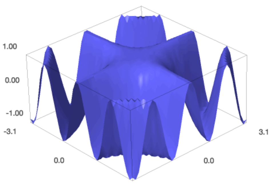
Fig. 41 The plot of the surface \(z = \cos(x y)\).

We observe that the plot is rather flat and this is considering the values for \(x\) and \(y\) range from \(-3.14\) to \(+3.xiv\), where as the \(\cos(\cdot)\) takes values between \(-ane\) and \(+1\). To make the plot less flat, nosotros alter the aspect_ratio and we make the plot spin, as follows:

                            plot3d              (              cos              (              10              *              y              ),              (              x              ,              -              pi              ,              pi              ),              (              y              ,              -              pi              ,              pi              ),              \              aspect_ratio              =              (              i              ,              i              ,              ii              ),              spin              =              one              )            

We can modify the viewing angle with the methods rotateX() and rotateZ() for example.

                            plot3d              (              cos              (              x              *              y              ),              (              x              ,              -              pi              ,              pi              ),              (              y              ,              -              pi              ,              pi              ),              \              aspect_ratio              =              (              ane              ,              1              ,              2              ))              .              rotateX              (              pi              /              ii              )              .              rotateZ              (              pi              /              4              )            

The result of the rotation of the viewing angles is shown in Fig. 42.

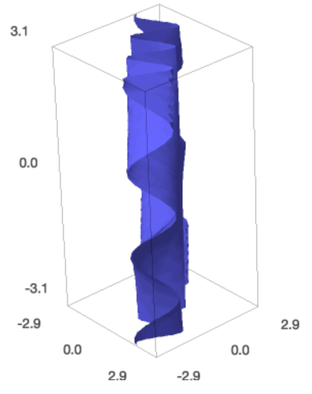
Fig. 42 The plot of the surface \(z = \cos(x y)\) with adjusted viewing angles.

By default, the value for opacity is 1, we tin can brand the plot more transparant by lowering that value. We can also increase the number of plot points.

                            plot3d              (              cos              (              ten              *              y              ),              (              ten              ,              -              pi              ,              pi              ),              (              y              ,              -              pi              ,              pi              ),              aspect_ratio              =              (              ane              ,              1              ,              two              ),              \              plot_points              =              [              60              ,              lx              ],              opacity              =              0.75              )              .              rotateX              (              pi              /              10              )              .              rotateY              (              -              pi              /              10              )            

Meet Fig. 43 for the corresponding picture.

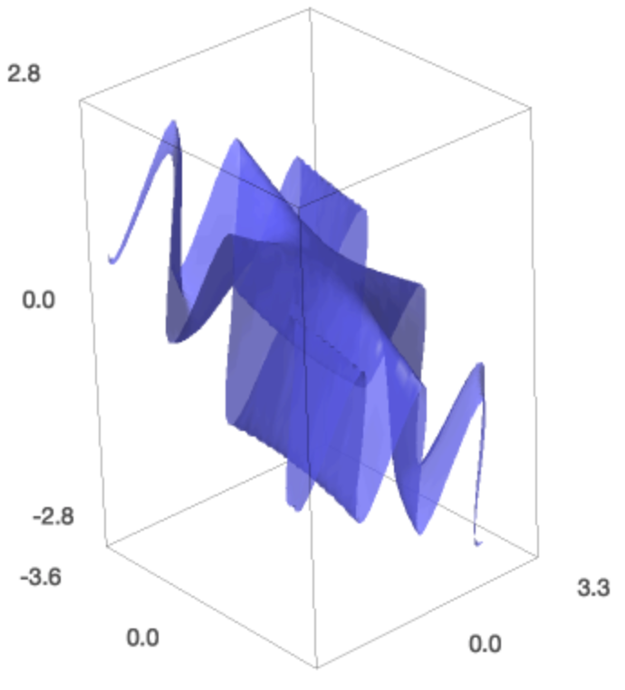
Fig. 43 The plot of the surface \(z = \cos(x y)\) with adjusted viewing angles, defined number of plot points, and an opacity factor.

Instead of trying to guess the best number of plot points, we can set adaptive to Truthful . Setting color to 'automatic' chooses a rainbow of colors, we tin set up the number of colors with num_colors .

                            plot3d              (              cos              (              x              *              y              ),              (              10              ,              -              pi              ,              pi              ),              (              y              ,              -              pi              ,              pi              ),              adaptive              =              Truthful              ,              \              aspect_ratio              =              (              i              ,              1              ,              2              ),              color              =              'automatic'              ,              num_colors              =              256              )            

The colorful plot is shown in Fig. 44.

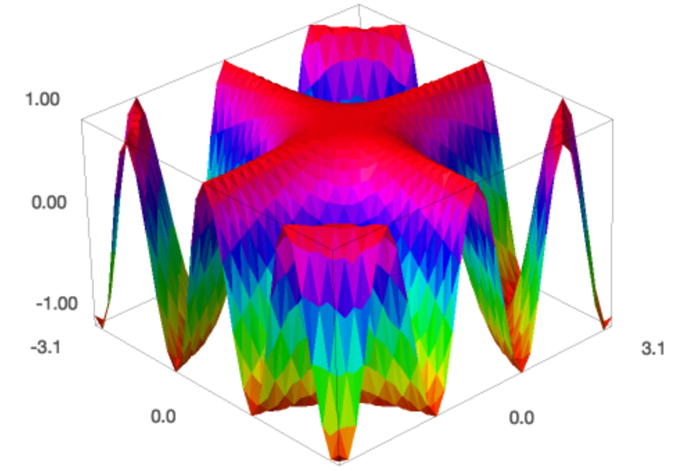
Fig. 44 The plot of the surface \(z = \cos(x y)\) with an adaptive choice of plot points and with many colors.

Surfaces may be given in parametric form by three expressions in two variables, say \(u\) and \(v\), as \(10 = f_x(u,v), y = f_y(u,five)\), and \(z = f_z(u,v)\). And so we utilise parametric_plot3d . The case below comes from the Sage documentation.

                            u              ,              5              =              var              (              'u, v'              )              fx              =              cos              (              u              )              *              (              4              *              sqrt              (              one              -              five              ^              2              )              *              sin              (              abs              (              u              ))              ^              abs              (              u              ))              fy              =              sin              (              u              )              *              (              iv              *              sqrt              (              one              -              v              ^              ii              )              *              sin              (              abs              (              u              ))              ^              abs              (              u              ))              fz              =              v              heart              =              parametric_plot3d              ([              fx              ,              fy              ,              fz              ],              (              u              ,              -              pi              ,              pi              ),              (              v              ,              -              one              ,              i              ),              \              color              =              'red'              )              .              rotateX              (              -              pi              /              9              )              .              rotateY              (              -              pi              /              2              )              .              rotateZ              (              pi              /              4              )              show              (              centre              ,              frame              =              False              )            

Detect how we can forbid the bounding box from actualization. The surface is shown in Fig. 45.

Fig. 45 The plot of a parametric surface.

Space Curves¶

A infinite curve is defined past a parametric plot of 3 functions in ane variable. For instance, the twisted cubic is defined by \(x = t, y = t^2, z = t^3\).

                            t              =              var              (              't'              )              twisted              =              (              t              ,              t              ^              two              ,              t              ^              3              )              parametric_plot3d              (              twisted              ,              (              t              ,              -              one              ,              ane              ))            

We can make the bend look carmine and thicker.

                            pt              =              parametric_plot3d              (              twisted              ,              (              t              ,              -              ane              ,              1              ),              colour              =              'red'              ,              thickness              =              five              )              bear witness              (              pt              )            

The result of the parametric_plot3d is shown in Fig. 46.

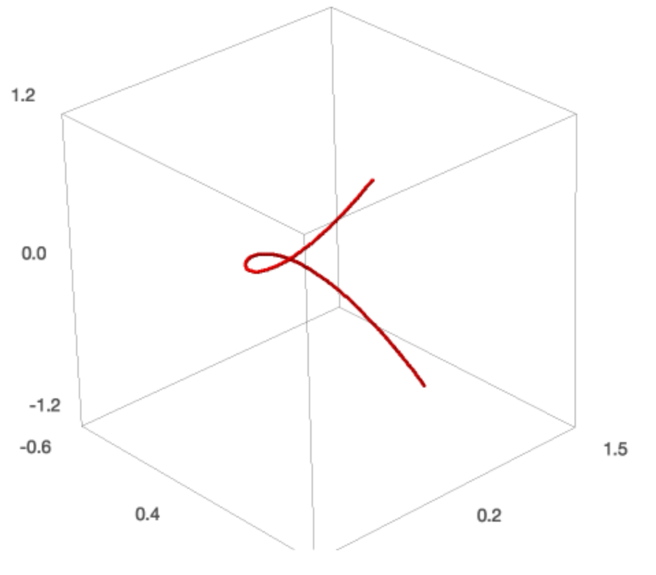
Fig. 46 A plot of the space curve \((t, t^2, t^iii)\), the twisted cubic.

In that location is a bounding box attribute associated to the plot.

We need to know the bounding box if we want to add to the plot, so we know which ranges for the iii coordinates to choose. The twisted cubic is the intersection of a parabolic and a cubic cylinder. The parabolic cylinder has its base of operations in the \((x,y)\)-plane and from the parametric representation of the twisted cubic \((10=t, y=t^2)\), we can derive the implicit equation as \(ten^two - y = 0\).

                            x              ,              y              ,              z              =              var              (              'x,y,z'              )              c2              =              implicit_plot3d              (              10              ^              ii              -              y              ,(              10              ,              -              1              ,              1              ),(              y              ,              0              ,              ane              ),              (              z              ,              -              one              ,              1              ))              show              (              pt              +              c2              )            

The result of the implicit_plot3d is shown in Fig. 47.

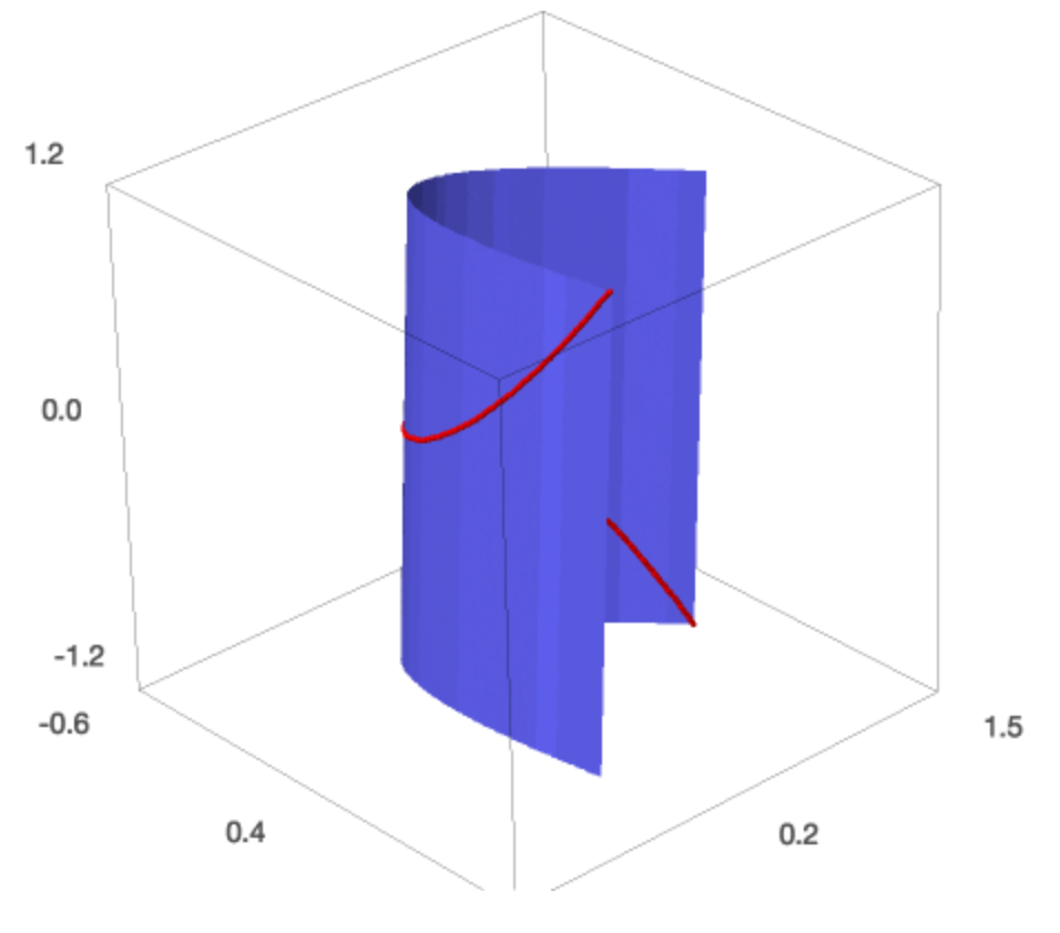
Fig. 47 The twisted cubic \((t, t^two, t^3)\) on the parabolic cylinder \(x^ii - y = 0\).

The cubic cylinder has its base in the \((10, z)\)-plane and its equation can be derived from the parameter representation for the twisted cubic, \((10=t, z=t^3)\) so the equation is \(x^iii - z = 0\).

                            c3              =              implicit_plot3d              (              10              ^              three              -              z              ,(              x              ,              -              i              ,              ane              ),(              y              ,              0              ,              ane              ),              (              z              ,              -              one              ,              1              ),              colour              =              'green'              )              evidence              (              pt              +              c2              +              c3              )            

Nosotros so see the two cylinders with the twisted cubic equally their intersection.

Four Dimensional Plots with Colormaps¶

With colormaps we can plot in 4 dimensions. Let us first explore the use of colormaps. Nosotros tin color surfaces with a colormap. As an example we have the Moebius strip. Starting time we plot it without color.

                            from              sage.plot.plot3d.parametric_surface              import              MoebiusStrip              ms              =              MoebiusStrip              (              3              ,              1              ,              plot_points              =              200              )              .              rotateX              (              -              pi              /              8              )              prove              (              ms              )            

The figure is shown in Fig. 48.

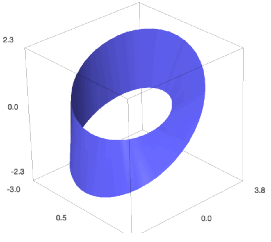
Fig. 48 The Moebius strip is a one-sided surface.

Now we apply a colormap.

                            cm              =              colormaps              .              ocean              def              c              (              ten              ,              y              ):              render              sin              (              x              *              y              )              **              ii              mscm              =              MoebiusStrip              (              3              ,              one              ,              plot_points              =              200              ,              colour              =              (              c              ,              cm              ))              .              rotateX              (              -              pi              /              eight              )              show              (              mscm              ,              frame              =              False              ,              viewer              =              'tachyon'              )            

The Moebius strip shown in colors is displayed in Fig. 49.

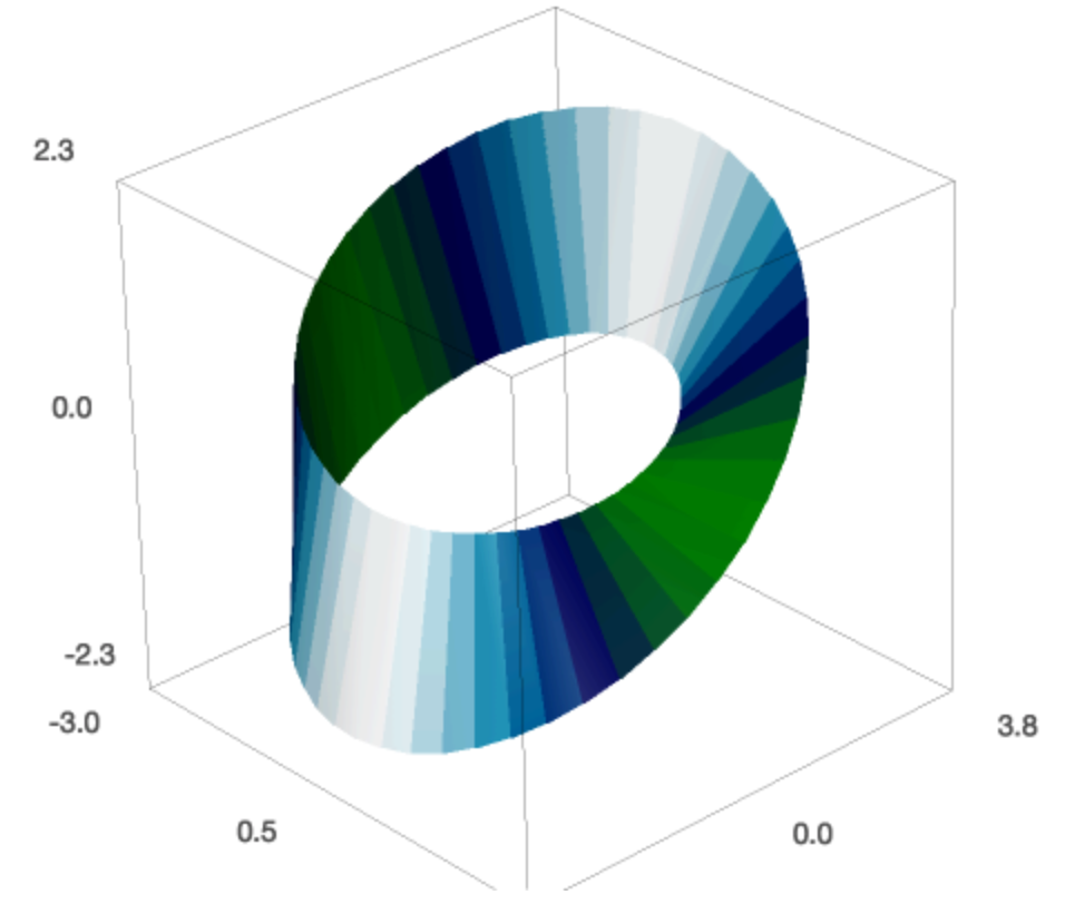
Fig. 49 A colored one sided surface, the Moebius strip.

We tin use colormaps to make four dimensional plots. Consider the cubic root of a complex number.

                            u              ,              v              =              var              (              'u,five'              )              w              =              u              +              I              *              five              z              =              westward              ^              three              x              =              real_part              (              z              )              y              =              imag_part              (              z              )            

We consider any complex number w . Considering u and v are real numbers, so we can simplify their real and imaginary parts.

                            D              =              {              real_part              (              u              ):              u              ,              imag_part              (              u              ):              0              ,              real_part              (              5              ):              v              ,              imag_part              (              v              ):              0              }              twenty              =              x              .              subs              (              D              )              yy              =              y              .              subs              (              D              )              print              twenty              print              yy            

and so we see u^three - iii*u*v^2 and 3*u^2*v - v^iii every bit the expressions for 20 and yy . We can now plot the surface using the expressions for twenty and yy every bit functions of u and v , just equally parametric_plot3d((xx, yy, u), (u, -1, 1), (v, -1, 1)) .

Why does this represent the cubic root? Well, the elevation of the surface is u , the real part of the circuitous number w nosotros started with. The twenty and yy are the real and imaginary parts of the z , where z was obtained by taking the number u + I*5 to the 3rd ability.

Going to polar coordinates produces a nicer plot.

                            r              ,              t              =              var              (              'r,t'              )              rt              =              {              u              :              r              *              cos              (              t              ),              v              :              r              *              sin              (              t              )}              px              =              twenty              .              subs              (              rt              )              py              =              yy              .              subs              (              rt              )            

and now we make the plot as

                            parametric_plot3d              ((              px              ,              py              ,              r              *              cos              (              t              )),              (              r              ,              0              ,              1              ),              (              t              ,              0              ,              2              *              pi              ),              adaptive              =              Truthful              )            

The plot is shown in Fig. 50.

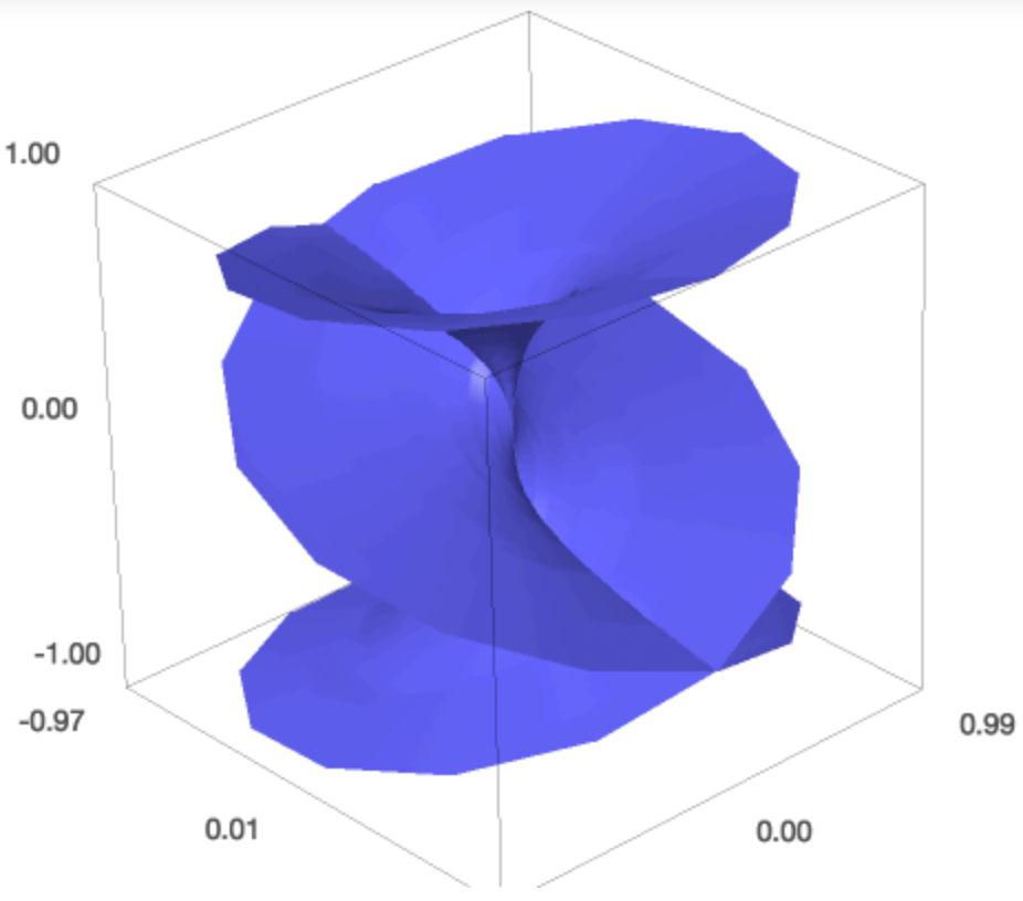
Fig. 50 A plot of the real role of the cubic root surface.

Now we would similar equally color to employ the imaginary part, v = r*sin(t) .

                            cm              =              colormaps              .              autumn              def              c              (              r              ,              t              ):              return              r              *              sin              (              t              )              cr              =              parametric_plot3d              ((              px              ,              py              ,              r              *              cos              (              t              )),              (              r              ,              0              ,              1              ),              (              t              ,              0              ,              2              *              pi              ),              \              adaptive              =              True              ,              color              =              (              c              ,              cm              ))              .              rotateX              (              pi              /              10              )              .              rotateY              (              -              pi              )              .              rotateZ              (              pi              /              ii              )              show              (              cr              ,              frame              =              False              ,              viewer              =              'tachyon'              )            

and this produces the plot shown in Fig. 51.

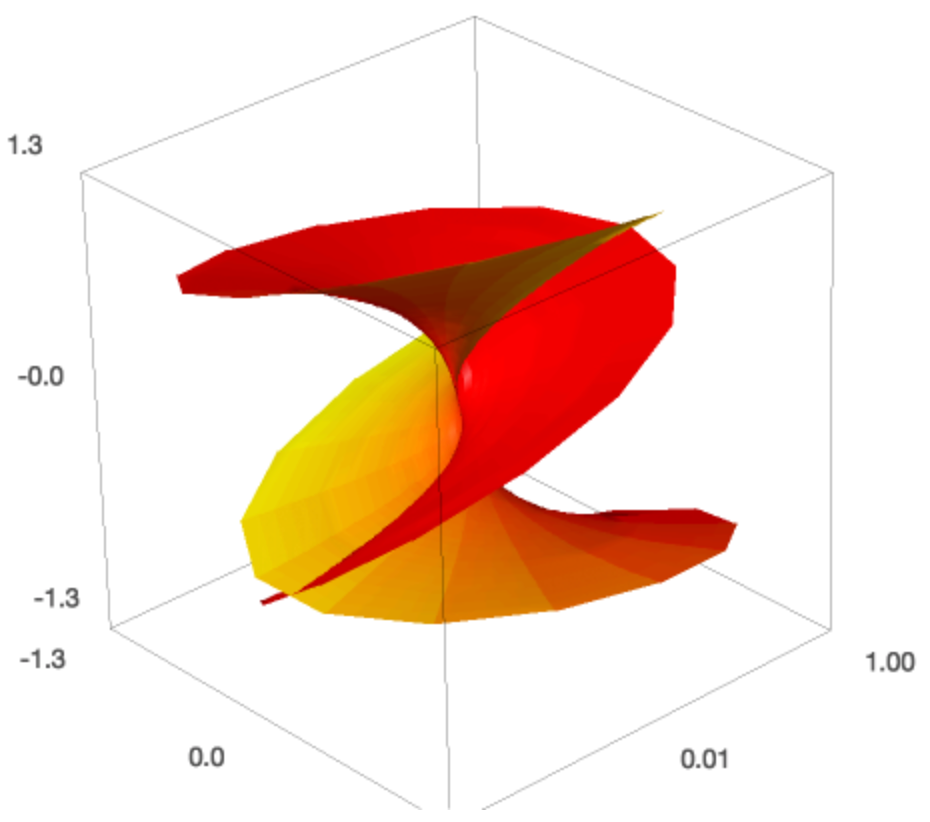
Fig. 51 The plot of a Riemann surface.

The height of the surface is the existent part and the colour of the surface represents the imaginary office of the cubic root. This is a four dimensional plot, as well called a Riemann surface.

Assignments¶

1. Consider \(h = two \cos(0.4x) \cos(0.4y) + 5 x y e^{-(x^2 + y^2)} + 3 east^{-((10-two)^two + (y-2)^2)}\). Choose appropriate ranges for \(x\) and \(y\) so that the plot of this surface shows iii peaks.
2. The Viviani curve is a infinite bend defined by \(x = \cos^ii(t)\), \(y = \cos(t) \sin(t)\), and \(z = \sin(t)\). Requite the SageMath command to plot this infinite curve.
3. The Viviani curve is defined equally the intersection of the sphere \(10^2 + y^2 + z^2 = ane\) and the cylinder \(x^two + y^2 = 1\). Plot the two surfaces and emphasize their intersection adding the result of the plot of the previous exercise.
4. A torus knot is defined by \(r = 2 + 4/5 \cos(7t)\), \(x = r \cos(4 t)\), \(y = r \sin(4 t)\), and \(z = \sin(7t)\). Plot this knot with SageMath.
5. Consider the surface defined by the equation \(f(x,y,z) = x^3 - y^2 - z^2 = 0\).
   1. Give the SageMath command to plot this surface, for \(x \in [0, 1]\) and for \(y, z \in [-1, 1]\). What do you run into at (0,0,0)? Draw.
   2. Supercede \(z\) past zero and transform the curve defined by \(f(x, y, 0) = 0\) into polar coordinates. Write the SageMath control to graph the bend in polar coordinates. Utilise skilful bounds for the range of \(t\).

francisfecid1968.blogspot.com

Source: https://homepages.math.uic.edu/~jan/mcs320/mcs320notes/lec26.html

Share this post